feeLLGood – Quick start guide

This guide is designed to help you get started with feeLLGood by performing a simple micromagnetic simulation. We assume that you have at least some basic knowledge of micromagnetism, that you are using a computer running Linux, and that you have some familiarity with the Linux command line and a text editor. The instructions below have been tested on an Ubuntu 22.04 system: you may have to adapt them if running a different flavor of Linux.

Before going through this guide, you should install feeLLGood on your computer. See the installation guide. In order to follow along, you should also install some extra tools that are useful for creating a mesh and viewing the simulation results:

sudo apt install python3-gmsh python3-numpy gnuplot paraview

Define the problem

The first step is obviously to define the problem we want to solve. For this guide, we will simulate a very small object over a very short time. This is intended to keep the simulation time short, as a more typical problem may require multiple days of computing time.

Our sample will be a magnetically soft cylinder of 32 nm height and 32 nm diameter, as depicted in the figure below. Its magnetization will be initially uniform, at 45° from the cylinder’s axis. We will look at its evolution with no applied magnetic field. For the material, we will use the parameters of permalloy: a magnetization of 1 T/µ₀ and exchange constant of 10 pJ/m. For the Gilbert damping constant, there is a wide spread in the values reported in the literature. We will choose α = 0.05, which is a value near the top of the range. This choice is meant to make the effects of the damping more obvious over a short simulation timespan. The simulation will only cover one nanosecond, which is just enough to see something interesting.

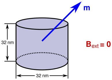
Although simple, this simulation can answer a couple of interesting questions. We expect an object of this size to be single domain, and its magnetization to evolve towards an easy direction of its shape anisotropy. What is this direction? We know an elongated rod would have its magnetization along its axis, and a flat disc would be magnetized in-plane. But what about such a cylinder, which has a height equal to its diameter? Will the magnetization turn towards the axis or away from it? The second question is about the uniformity of the magnetization. This object is small enough to be single domain, yet too large for the magnetization to be completely uniform. How far from uniform will the magnetization be?

The simulation we are going to perform will show the dynamic evolution of the magnetization starting from an out-of-equilibrium state. If we were only interested in the equilibrium configuration, we would use an unrealistically large damping constant, like 0.5 or 1. Then, the equilibrium would be reached faster, but the evolution would be non-physical.

Create the mesh

The second step is to build a mesh for the geometry of our magnetic object. Properly defining and meshing the geometry of a sample is a complex topic, far beyond the scope of this quick-start guide. But since we need a mesh anyway, we will take a shortcut. FeeLLGood ships a Python module called “meshMaker”, which can mesh simple geometries. We will use the Cylinder function from this module to get a mesh of our cylinder.

Let’s start by creating a directory for holding the files of the simulation:

$ mkdir quick-start
$ cd quick-start

Now, with your editor of choice, create this Python script and save it as “mksample.py”:

from feellgood.meshMaker import Cylinder

height = 32          # we use nanometers
radius = height / 2  # so diameter = heigh
elt_size = 4         # typical element size
surface_name = "surface"
volume_name = "volume"

# Create the mesh and save it in the file "cylinder.msh".
mesh = Cylinder(radius, height, elt_size, surface_name, volume_name)
mesh.make("cylinder.msh")

In order for a mesh to properly sample the magnetization configuration, its average element size has to be smaller than the material’s exchange length, although it doesn’t need to be much smaller. As the exchange length of permalloy is about 5 nm, we have chosen 4 nm for the element size.

We have to name every surface region and volume region defined in our mesh. Here, as we have a simple object with only one region of each kind, we simply named the regions “surface” and “volume”. If we were meshing a complex system consisting of multiple regions of different materials, we would have to get more creative in the naming.

Now run the script:

$ python3 mksample.py
Generated cylinder.msh: 629 nodes, 2361 tetrahedra, 880 triangles

Here we are: we have our mesh. It is a cylinder, centered at the origin, with its axis along the z axis of the coordinate system.

Write the settings file

Now, we have to write a YAML file with all the information about our problem that is not already in the mesh itself. As there are many parameters to set, and the syntax is quite strict, it is easier to start from a template. We can ask feeLLGood to create this template for us, pre-filled with all its default settings:

feellgood --print-defaults > settings.yml

Now, open this file with your favorite text editor. It is heavily commented, and we recommend you carefully read all those comments at least once. Then, we can remove everything that is not needed: the comments and the settings that we leave at their default values, and then add our own comments and our own settings. While doing so, mind the indentation, as it is meaningful to the YAML syntax. In the end, the file should look like this:

# Simulate a 32×32 nm permalloy cylinder.

outputs:
  final_time: 1e-9      # simulate one nanosecond

mesh:
  filename: cylinder.msh
  length_unit: 1e-9     # mesh unit is nanometers
  volume_regions:
    volume:             # high-damping permalloy
      Ae: 1e-11         # exchange constant
      Js: 1             # µ₀Ms
      alpha_LLG: 0.05   # Gilbert damping
  surface_regions:
    surface:

initial_magnetization: [1, 0, 1]  # at 45° from z axis

Bext: [0, 0, 0]         # no applied field

Here we have removed most of the settings, as the defaults are good enough for this simple problem. When dealing with a more substantial simulation, we recommend you first do shorter simulations while tweaking the two nb_threads parameters and the parameters in the time_integration section. By doing so you will be able to optimize the speed of the computation.

There are a few parameters in the YAML file above that we have left at their default values: the mesh length unit, the applied field, and two material parameters. Although we could remove these parameters from the file, we have chosen to leave them there because we feel they are essential to the definition of the problem, and the above file serves also to document our choices.

Note that feeLLGood requires us to list all the surface and volume regions of our object, even if we leave all the corresponding parameters at their default values. Hence the presence of the surface region named “surface” in this file. Note also that the initial magnetization vector we provided is not normalized: we will let feeLLGood normalize it for us.

If you do not feel confident in the syntax of your settings file, you can ask feeLLGood to check it:

$ feellgood --verify settings.yml

FeeLLGood will then read the file, merge it with its built-in defaults, and print the resulting complete configuration.

Run the simulation

Once the settings file is ready, invoke feellgood with the name of the file as its sole argument:

$ feellgood settings.yml
        ┌────────────────────────────────┐
        │           feeLLGood            │
        │      CNRS Grenoble – INP       │
        │ https://feellgood.neel.cnrs.fr │
        └────────────────────────────────┘
feeLLGood version: 0.7.1-26-g80501b5
process ID:        2563864
random seed:       468240227
settings file:     settings.yml
mesh file:         cylinder.msh
output directory:  . (already exists)
progress:          100.00%  

Time step statistics:

    time steps       count       dt [*]          dumax [*]
    ──────────────────────────────────────────────────────────
    successful        2232   3.98e-13 ± 0.67   4.06e-03 ± 0.52
    failed               0

    [*] ranges given as (geometric mean) ± (relative stddev)

Computing time:

    total: 279.181 s (4.65302 min)
    per time step: 0.125081 s

Now we have some new files in our working directory:

• cylinder.evol contains global quantities sampled at regular time intervals. We are mostly interested in the averaged reduced magnetization.

• cylinder_iter*.sol are snapshots of the magnetization configuration. The numbers in the file names are time step numbers. The actual times are written as comments near the top of the files.

All these files are plain text, tab-separated numerical values. They have comments near the top, which are signaled by a # character at the beginning of the line.

Visualize the results

Let's start by looking at the evolution the average magnetization. For this, you can use whatever plotting program you are most comfortable with. Here, for the sake of illustration, we will use gnuplot.

First, we plot the three components of the magnetization (second, third and fourth columns of the file cylinder.evol) against time (first column):

$ gnuplot

        G N U P L O T
        [standard Gnuplot blurb...]
gnuplot> set style data lines
gnuplot> plot 'cylinder.evol' using 1:2 title 'm_x', \
> '' using 1:3 title 'm_y', \
> '' using 1:4 title 'm_z'

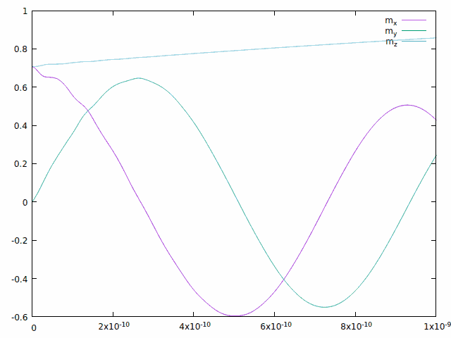
Looking at the x and y components, we see they precess counterclockwise when seen from above, which is an indication that the effective field is pointing upwards. This is confirmed by the z component increasing: the magnetization precesses while converging towards the axis of the cylinder. We now have the answer to our first question: our cylinder has an easy-axis type of shape anisotropy. We could fit the precession frequency if we wanted to evaluate the strength of this anisotropy.

On top of this damped precession, there are some fast oscillations mostly visible on the x component during the first hundred picoseconds. We suspect this is due to non-uniform modes: the magnetization rearranging itself into a not quite uniform configuration. We can confirm this suspicion by plotting the modulus of the average reduced magnetization:

gnuplot> plot 'cylinder.evol' using 1:(sqrt($2**2+$3**2+$4**2))

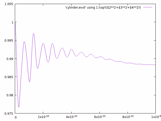
This plot confirms the suspicion, and also provides the data needed to answer our second question: how far from uniform is the magnetization? This is time-dependent, but we can nevertheless put some number on the non-uniformity at the final time, which seems to be not too far from the long-time asymptote.

Let's call θ the angle by which the local magnetization deviates from its average direction. By assuming θ is small, Taylor-expanding cos θ to second order, and averaging over the sample, we write the modulus of the average reduced magnetization as:

From this, the root-mean-square deviation is

At the end of the simulation, we have |⟨m⟩| ≈ 0.9883, from which it follows that the magnetization deviates from a uniform configuration by an RMS angle of about 0.153 rad, or 8.76°.

Now, getting a number is nice, but we would also like to see what the actual magnetization configuration looks like. For this, we will use ParaView. We first have to convert the data into a format that ParaView can understand, namely VTK. The conversion is performed by the convert2vtk script, which lives in feeLLGood’s “tools” directory. The script parameters are the file name of the mesh and the file name of the snapshot we want to convert. Let's take a look at the very last snapshot:

$ tools/convert2vtk cylinder.msh cylinder_iter2000.sol
cylinder_iter2000.vtu saved as 3D vectors, using  [1, 2, 3]  columns

We can now visualize the magnetic configuration with ParaView:

$ paraview cylinder_iter2000.vtu

The display is initially empty. In order to see the vector field, we have to:

1. click on the “Apply” button in the Properties tab

2. click on the Glyph icon on the third toolbar

3. click again on “Apply”

4. select “Vectors_”, then “X” in the combo boxes

The relevant widgets are highlighted in the screenshot below:

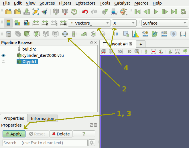
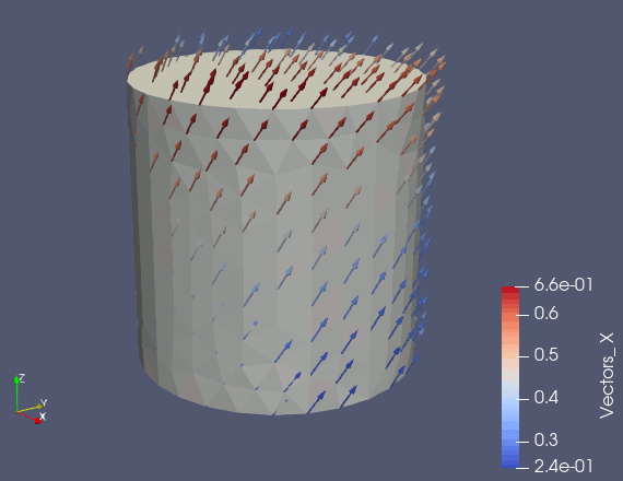
Step 4 is not strictly required, but it makes the non-uniformity more obvious. We can now use the mouse to turn the object around and see the vector field from different angles:

Conclusion

Solving a problem of micromagnetism with feeLLGood consists of three main steps:

1. build the mesh

2. use feeLLGood to do the actual simulation

3. analyze the results

Steps 1 and 3 are complex, and require some experience in order to be performed properly. However, these steps fall outside the scope of the feeLLGood project. For step 2, the main difficulty is correctly filling the settings file that controls the feeLLGood simulation. Please, refer to the reference section of the documentation for the precise meaning of each of the parameters defined in this file.