feeLLGood – Phase diagram of nanodots

The lowest-energy state of a magnetic nanodot (a small disk-shaped magnet) can be either a magnetic vortex, where the magnetization wraps around the disk, or a single domain, where the magnetization is mostly uniform. Both configurations are at least metastable over a wide range of parameters. Which of these is the lowest energy state depends on the dimensions of the disk (diameter and thickness) relative to the exchange length of the magnetic material.

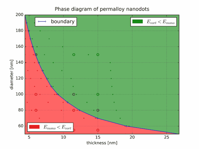
In this example we would like to determine, for a disk of permalloy within a range of sizes, which of these states is the most stable (has the lowest energy), as a function of the disk dimensions. The goal is to compute a phase diagram similar to the one experimentally determined in this paper: R. P. Cowburn, D. K. Koltsov, A. O. Adeyeye, M. E. Welland, and D. M. Tricker Single-Domain Circular Nanomagnets, Phys. Rev. Lett. 83, 1042 (1999).

This example is based on work done by Shriraj Hegde during the spring 2023, as he was an intern at Spintec.

Problem definition

The sample is a disk of permalloy with the following material properties:

Ae: 1.3e-11
Js: 1.00531

There is no anisotropy, and no applied field. Given the disk dimensions, we want to know which of the two states has the lowest energy. The expectation is that the vortex state will be the most stable on large and thick disks, whereas on smaller disks it will be the single-domain state.

In order to build a phase diagram we will determine, for a set of diameters ranging from 50 nm to 200 nm, what is the threshold thickness above which the vortex state is most stable.

In order to compute the energy of a given state, we will initialize the magnetization configuration with an ansatz of that state, i.e. an initial guess close to the desired state. We will then let the system relax until it finds its local energy minimum.

Initial states

As the single-domain state is close to uniform, its ansatz will be a uniform magnetization along the x direction:

For the vortex state, we will use a counterclockwise configuration, with the vortex core along +z. The simplest such ansatz is possibly this:

where r is a parameter that can be interpreted as the radius of the vortex core. This parameter should be chosen in a way that minimizes the ansatz energy. The reason is that, the less energy the system has to dissipate, the less likely it is to relax towards a very different state.

In order to optimize for r, we choose a 100×10 nm disk as our “typical” sample. This size is (logarithmically) in the middle of our diameter range and, as we will see later, very close to the boundary we are interested in. Here is the Python script that creates the mesh for this disk:

# Mesh a 100 × 10 nm nanodot.

from feellgood.meshMaker import Cylinder

diameter = 100
thickness = 10
elt_size = 4
radius = diameter / 2
mesh = Cylinder(radius, thickness, elt_size, "surface", "volume")
mesh.make("nanodot-100x10.msh")

The element size has been chosen to be somewhat smaller than the exchange length which, for these material parameters, is about 5 nm.

And here is the settings file for a feeLLGood run:

outputs:
  file_basename: core-size
  evol_columns: [E_tot]
  final_time: 0
  mag_config_every: false

mesh:
  filename: nanodot-100x10.msh
  volume_regions:
    volume:
      Ae: 1.3e-11
      Js: 1.00531
  surface_regions:
    surface:

initial_magnetization: [-y, x, 4e-9]  # 4e-9 is just an example

Note the parameter outputs.final_time = 0. This instructs feeLLGood to quit after writing a single data line to the file core-size.evol, which corresponds to the initial state. In this case, the file will contain a single line (t = 0) and a single column (E_tot). That is, it will have only the initial energy. Note also that the initial magnetization vector is not normalized: feeLLGood will take care of the normalization.

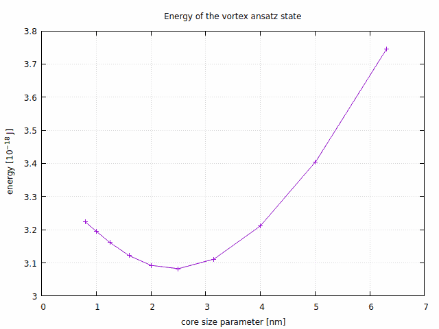
The same computation can be repeated for a selection of core radii (this is easy to automate), which leads to the following dependence of the ansatz energy on the core radius:

Fitting a quadratic polynomial to the three lowest-energy points gives an optimal core size of 2.4 nm. This may seem unreasonably small, given that the typical mesh element size is 4 nm. The relaxed core, however, is significantly wider. The reason we get such a small size is because this ansatz has a core with much wider tails than the actual relaxed state.

Relaxation time

Building the phase diagram will require many hours of computing time. In order to keep this computing time reasonable, we should optimize the simulated relaxation time: it should be large enough to let the system get very close to its final energy, but no larger than needed.

In order to choose a suitable relaxation time, we perform a couple of simulations (one for each state) with a simulation time that is clearly longer than needed, namely 5 ns. Here is the feeLLGood settings file for the single-domain state:

outputs:
  file_basename: single_domain
  evol_columns: [t, <Mx>, <My>, <Mz>, E_tot]
  final_time: 5e-9
  mag_config_every: false

mesh:
  filename: nanodot-100x10.msh
  volume_regions:
    volume:
      Ae: 1.3e-11
      Js: 1.00531
      alpha_LLG: 0.5
  surface_regions:
    surface:

initial_magnetization: [1, 0, 0]

Note the alpha damping constant: this very large value does not give realistic dynamics, but is suitable for quickly relaxing to the closest energy minimum.

The settings file for the vortex state is identical to the one above but for these two parameters:

outputs:
  file_basename: vortex
initial_magnetization: [-y, x, 2.4e-9]

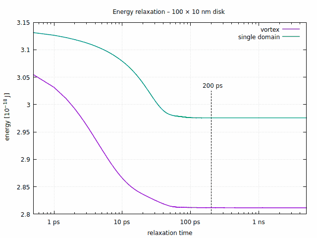
Here is the evolution of the energy for both states, plotted against logarithmic time:

Although the disks are mostly relaxed after 100 ps, we choose 200 ps as the relaxation time in order to keep some safety margin.

Finding the boundary

The boundary between the single-domain and the vortex states is found by stepping through the diameter range and, for each diameter, finding the thickness that solves the equation:

This is accomplished by the Python script provided at the end of this page, which is generously commented, and should be mostly self-explanatory. There are, however, a few points worth discussing here.

The function make_mesh() defines the typical element size as follows:

elt_size = min(4, thickness / 2)

This is 4 nm, unless the disk is very thin, in which case the element size is half the thickness. The reason for this is that, in order for the finite element method used by feeLLGood to give accurate results on thin films, there should be at least two elements across the film thickness.

The script has a few calls to os.makedirs() and os.chdir(). These are intended to organize the large amount of generated content in a directory structure like this:

.                   # initial working directory
└── data            # a single subdirectory for all the generated data
    ├── 50.0x3.000  # a subdirectory for each disk size
    │   ├── nanodot.msh              # the meshed sample
    │   ├── single_domain.json       # settings file for single-domain
    │   ├── single_domain.evol       # evolution of single-domain
    │   ├── single_domain_iter*.sol  # a few magnetization snapshots
    │   ├── vortex.json              # settings file for vortex
    │   ├── vortex.evol              # evolution of vortex
    │   └── vortex_iter*.sol         # a few magnetization snapshots
    └── ...         # more subdirectories for other sizes

Near the end of the script, there is this line:

critical_thickness = optimize.brentq(energy_difference, ...)

This is where the equation \(E_\text{single-domain} - E_\text{vortex} = 0\) is solved for. This invokes Brent’s root-finding algorithm, as implemented by the optimize.brentq() method from the SciPy scientific computing library.

Below is the full Python script used to compute the phase boundary:

import os
import json
import numpy as np
from scipy import optimize
from feellgood.meshMaker import Cylinder

# Range of nanodot dimensions to be explored (nanometers).
diameter_range = [50, 200]
diameter_step = 10
thickness_range = [3, 30]

# How long to relax (seconds).
simulation_time = 2e-10

# Material parameters.
material = {
    "Ae": 1.3e-11,
    "Js": 1.00531,
    "alpha_LLG": 0.5
}

# Initial magnetization configurations.
initial_magnetizations = {
    "single_domain": [1, 0, 0],
    "vortex": ["-y", "x", 2.4e-9]  # CCW vortex, with core along +z
}

# Build a mesh of the given dimensions, named "nanodot.msh".
def make_mesh(diameter, thickness):
    radius = diameter / 2
    elt_size = min(4, thickness / 2)
    mesh = Cylinder(radius, thickness, elt_size, "surface", "volume")
    mesh.make("nanodot.msh")

# Read the relaxed energy off the given evol file.
# It is the last field (E_tot) of the last line (final time).
def read_energy(evol_file_name):
    return np.loadtxt(evol_file_name)[-1][-1]

# Simulate "nanodot.msh" in the given mode, which should be either
# "single_domain" or "vortex". Return the final energy.
def run_sim(mode):
    settings = {
        "outputs": {
            "file_basename": mode,
            "evol_columns": ["t", "<Mx>", "<My>", "<Mz>", "E_tot"],
            "final_time": simulation_time
        },
        "mesh": {
            "filename": "nanodot.msh",
            "volume_regions": { "volume": material },
            "surface_regions": { "surface": {} }
        },
        "initial_magnetization": initial_magnetizations[mode]
    }
    settings_file = f"{mode}.json"
    json.dump(settings, open(settings_file, "w"), indent=4)

    os.system(f"feellgood {settings_file}")

    return read_energy(f"{mode}.evol")

# Run the simulations for both modes on the given dimensions, while
# storing the generated files in a dedicated directory.
# Return the final energies as a tuple (E_single_domain, E_vortex).
def run_size(diameter, thickness):
    dirname = f"{diameter:.1f}x{thickness:.3f}"
    os.makedirs(dirname, exist_ok=True)
    os.chdir(dirname)
    os.system("rm -rf *")  # clean the directory if not empty
    print(f"\n*** Starting D = {diameter:.1f}, t = {thickness:.3f}\n")
    make_mesh(diameter, thickness)
    print()

    E_single_domain = run_sim("single_domain")
    E_vortex = run_sim("vortex")

    os.chdir("..")  # get back to previous directory
    print(f"\nDone D = {diameter:.1f}, t = {thickness:.3f}")
    return (E_single_domain, E_vortex)

# Build two files:
# - results.txt: one line for every simulated size:
#   (thickness, diameter, E_single_domain, E_vortex)
# - boundary.txt: one line for every diameter:
#   (critical_thickness, diameter)
def main():
    # Store everything within a "data" subdir of the current directory.
    os.makedirs("data", exist_ok=True)
    os.chdir("data")

    # Run the simulations.
    results = []
    boundary = []
    all_diameters = np.arange(
        diameter_range[0],
        diameter_range[1] + diameter_step/2,
        diameter_step)
    for diameter in all_diameters:
        def energy_difference(thickness):
            E_single_domain, E_vortex = run_size(diameter, thickness)
            results.append([thickness, diameter, E_single_domain, E_vortex])
            return E_single_domain - E_vortex

        critical_thickness = optimize.brentq(energy_difference,
            thickness_range[0], thickness_range[1], rtol=1e-4, xtol=1e-2)

        boundary.append([critical_thickness, diameter])

    # Save the results.
    np.savetxt("results.txt", results,
        header="columns: thickness diameter E_single_domain E_vortex")
    np.savetxt("boundary.txt", boundary,
        header="columns: thickness diameter")

if __name__ == "__main__":
    try:
        main()
    except KeyboardInterrupt:
        exit()

And here are the final results, plotted as a state diagram. The blue line is the boundary, the small dots are the sizes for which the energies have been computed, and the circles show, for comparison, the experimental data of Cowburn et al.. In this diagram, the red color means single domain, whereas green stands for the vortex state.